SQL Server supports three physical join operators: Nested Loops, Merge and Hash.
The hash join works well for large sets of data. The hash join has two phases, the build and probe. First in the build phase, the rows are
read from the first table and hashes the rows based on the join keys and creates has table in memory. The second phase, the probe phase, the
hash join reads all the rows from the second table and hashes these rows based on the same join keys. The hash join then returns the
matching rows.
In pseudo-code, it shall look something like the following.
for each row Row1 in the build Table
begin
perform hash value calc on Row1 row join key
insert Row1 row into hash bucket
end
for every row Row2 in the probe table
begin
calc the hash value on row Row2 join key
for every row Row1 in the hash bucket
if row Row1 joins with row Row2
return (row Row1, row
Row2)
end
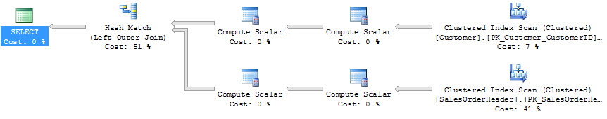
Below is an example of a select statement in which the optimizer should use a merge join operator.
select * from AdventureWorks.Sales.Customer c
left join AdventureWorks.Sales.SalesOrderHeader soh
on c.CustomerID = soh.CustomerID
SQL Server tries to use the smaller of the two tables as the build table. SQL Server does this to try and reserve precious memory. While
SQL Server attempts a best guess at guessing the amount of memory needed, if SQL has guessed to low it will spill out to tempdb to continue
joining for the hash join operation.